(Note:) I’m new to Jekyll and haven’t yet figured out how to escape parentheses [duh!]. So instead of parentheses I’ve been forced to use square brackets throughout…
As some of you may know, my wife and I recently spent a few months traveling in South America. We did the southernmost part of our trip - Chile and Argentina’s Patagonia - driving a car, which we bought in Santiago, Chile. As a sidenote for those who may be interested, Chile happens to be the only South American country at the time of writing this post that is somewhat friendly to foreigners buying cars and bringing them out of the country.
Buying a used car is always a risky business, particularly in a foreign country that you don’t know well. One of the obvious potential risks is that of overpaying, and since we had a lot of time to kill in Santiago while we were waiting for a strike to end, I decided to do a little bit of research on used car prices for the makes and models we were interested in.
What started like a small spreadsheet project ended up becoming a little more involved: I built a web scraper on R to download the prices of the listings from a couple of chilean websites, as well as a small shiny app to display and filter the results that were more relevant (you can find the whole project’s source code here: github.com/atibaup/chileConCars.)
In this blog post, I wanted to share some of the analysis that I did on the used car data, which turned out to be a pretty good used case for a class of models that I like: Mixed Effects Models.
Dataset
The dataset, which we obtained by scraping chileautos.cl and yapo.cl, contains 4213 samples of used cars with 17 features for each sample: “Nombre”, “Año”, “Fecha”, “URL”, “Código”, “Kilómetros”, “Precio”, “Precio.anterior”, “Tipo.de.vehículo”, “Combustible”, “Transmisión”, “Edad”, “Precio.USD”, “Kilómetros.miles”, “make”, “model”, “source”.
The breakdown of samples by make and model is shown below. It’s not surprising to see some of expensive models at the end of the list, but I was suprised by the huge lead in popularity that Suzuki’s got over its competitors. Or is it just that everybody’s trying to sell their Suzukis while other makes’ owners keep their cars throughout their lifetime?
| Suzuki GrandNomade | Suzuki GrandVitara | Honda CR-V | Toyota 4Runner | Nissan X-Trail | Mitsubishi Montero | Nissan Pathfinder | Toyota LandCruiser |
|---|---|---|---|---|---|---|---|
| 37.9 % | 16.8% | 11.9% | 8.8% | 8.2% | 7.5% | 5.7% | 3.1% |
In Chile, used cars tend to have automatic transmission, but manual cars are not far behind:
| Automático | Manual | NA’s |
|---|---|---|
| 50.2% | 40% | 9.7 % |
And unsurprisingly, Gas [Bencina] is a lot more popular than Diesel:
| Bencina | Diesel | Gas | Otros |
|---|---|---|---|
| 95.1% | 4.7% | 0.1% | 0.0% |
We can also look at the statistics of some of the features of interest, like the mileage [Kilómetros], the age [Edad] and the price in USD. The next figure shows the histograms and density estimates for each of these variables, segmented by model [the row order for each column is descending in the mean of the column’s variable]:
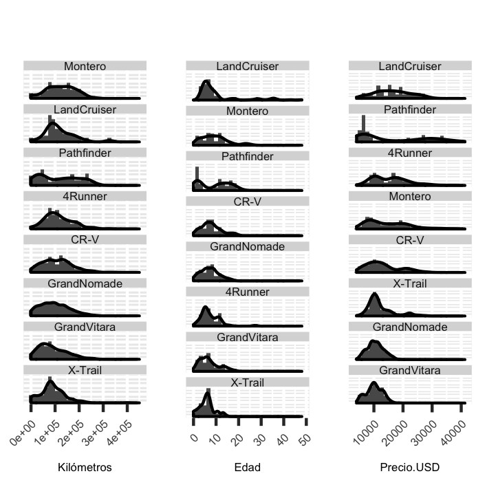
We can see that most used cars have around 100,000km under their hoods, and their ages are concentrated around the 10 years mark. Not surprisingly, models that are well-known to be very robust like the Mitsubishi Montero or the Toyota Landcruiser display a larger mileage and age spread, with some of the listings running well over 300,000kms. So if you’re thinking about driving 7 times around the world at the equator, you may want to consider one of those two!
The price statistics above also give a sense of the type of car that one can get for a given budget. For example, for a 10,000USD investment, we’re better off looking for a Suzuki Grand Nomade or a Honda CR-V than a Toyota Land Cruiser or a Toyota 4Runner, since the number of listings for the latter two for that price range is quite small.
Perhaps the most interesting feature is the bi-modality in the distribution of prices for some of the models [e.g. Pathfinder, 4Runner], which I found out to be largely explained by the bi-modality in the distribution of ages of the same segment.
Estimating depreciation rates
Since our main motivation for purchasing a car was to travel with it for a few months, we knew that we would be selling at the end. A natural question to ask then is how much will the car depreciate by the time we sell it, since this can inform our decision to choose one model or the other. We can try to estimate the [listing price] depreciation rate from the listing data for each car model via a simple additive regression model of the form:
$\log p = \mu_p + f_1(a) + \sum_{j>1} f_j\left(x_j\right) + \epsilon$
where $p$ is the listing price, $a$ is the age, the $x_j$’s are other relevant price-predicting features [e.g. transmission type, trim, fuel, etc], $f_j$ are regression functions, \(\epsilon\) is i.i.d. error. Assuming that the variables $x_j$ do not depend on the age variable $a$, we can obtain an estimate of the depreciation rate for each model as:
$\frac{\partial \log p}{\partial a} = \frac{\hat{f}_1}{\partial a} $
where $\hat{f}_1$ is the estimate of the regression function modeling the dependency between price and age.
This approach has one important shortcoming: It treats each car model independently, which given the scarcity of samples for some of the car models [see Toyota Land Cruiser or Nissan Pathfinder’s in the table above] may not be a great idea. For example, the depreciation rate for the Pathfinder would be estimated with only 130 samples, while the GrandNomade’s would be estimated with nearly 1600 samples, without leveraging the fact that all of these samples share a commonality: they all correspond to listing prices of SUV type cars, with 4 wheels, one steering wheel, and so on and so forth.
An alternative to this naive approach of treating each car model independently is to explicitly introduce a mechanism to pool information from samples across all car models. One such mechanism is provided by Mixed Effects Models [MEM], which we will consider here in a simplified log linear setting first. In this model, the response $p$ is a linear function of age and other variables,
$\log p = \mu^j_p + a\alpha^j + \mathbf{x}^T \beta^j + \epsilon$
where $j$ indexes the parameters corresponding to the $j$-th model. So far this is the same setup as the previous one, only that we have limited the class of functions to linear ones. In this model, however, instead of letting each tuple $(\mu^j_p, \alpha^j)$ be fitted independently for each car model, we assume that they are random samples drawn from a common distribution, which to simplify things we will assume is a multivariate Gaussian:
$(\mu^j_p, \alpha^j) \sim \mathcal{N}\left(\left(\bar{\mu}_p, \bar{\alpha}\right), \Sigma\right)$
Additionally, if $\epsilon$ is also normal, we have:
$\log p \left| \alpha^j, \mu^j_p \sim \right. \mathcal{N}\left(\mu^j_p + a\alpha^j + \mathbf{x}^T \beta^j, \sigma_\epsilon^2\right)$
The two last equations define a one-level hierarchical model, which imposes that all samples from the same car model share the same intercept and depreciation rate. The difference between the intercept and the depreciation rates of two different models is controled via the diagonal elements of $\Sigma$, which is estimated from the data. The name Mixed Effects Model comes from the fact that the model has a “random effect” component, corresponding to the $\mu^j_p$ and $\alpha^j$ covariates, as well as a “deterministic effect” component, corresponding to the $x^j$ covariates.
Let’s have a look at the results we obtain when fitting this simple MEM to our dataset. In our experiment, we use transmission type, fuel and mileage as additional covariates [the $x^j$’s in the equations above], and we fit the model using R’s (lmer) package. For comparison, we also fit the naive linear regression model to each model’s data. The next figure shows the predicted prices vs. age for each car model, when leaving the other covariates fixed. The original data points are shown in the background, however, the discrepancy to the fitted log-linear curve has to be taken with a grain of salt since we haven’t adjusted the data points to substract the effect from the other covariates [transmission, fuel]. Also shown in each plot’s header are the depreciation rates under the Mixed Effects [MEM] and the Fixed Effects [FE] models.
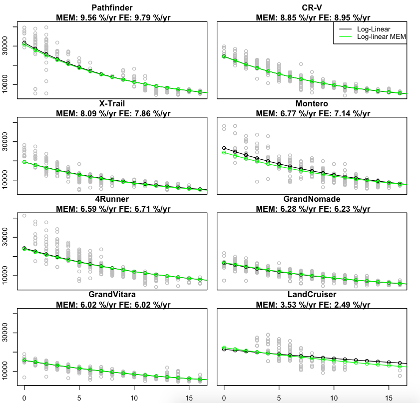
It is already clear from the plots that the difference between the estimates of each of the two approaches is not large, an observation that is supported by the small variance estimated for the random effect (\frac{\sigma_\alpha}{\mu_\alpha} = 0.28.) An interesting observation that we derive from the use of random effects is that the correlation between $\mu^j_p$ and $\alpha^j$ is around -0.5, which seems to imply that more expensive cars have smaller depreciation rates.
Also notable are the effects of the type of transmission and fuel on price. According to the MEM log-linear fit, a car with Manual transmission is valued at about 5% less than an Automatic one. On the other hand, Diesel models are about 15% more expensive than Gasoline ones [this is not suprising given the huge price difference in favor of Diesel fuel in Chilean gas stations, as well as the better fuel economy of Diesel engines].
One would be too quick to dismiss the utility of the MEM model given these results, especially after looking at the residual vs. fitted diagnosis plot for this log-linear MEM model:
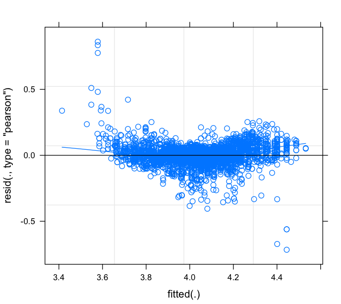
The residuals display a strong dependency to the fitted values and hence the log-linear model may be struggling to fit the data’s more complex non-linearities. We will see what we can do in the next post, where we will use polynomial splines within a Mixed Effect Model to better understand each car’s depreciation behavior. Stay tuned!