I ended my last post commenting on the poorness-of-fit of the log-linear Mixed Effects [(ME)] model fitted to the Chilean used car dataset. The residual vs. fitted plot seemed to indicate that there was an underlying non-linearity in the log-scale that the log-linear model wasn’t able to capture. In this post I’ll explore a few basis function based models that do a better job at fitting the data, and I’ll comment on the difficulty of estimating confidence intervals in Mixed Models using the (lme4) R package.
Linear non-linear models
All the models we consider next are (linear) in their parameters but model (non-linear) relationships between the covariate and the response variable, hence the catchy section title. In the context of used car price modeling, we had started from a generic additive regression model:
$\log p = \mu_p + f_1(a) + \sum_{j>1} f_j\left(x_j\right) + \epsilon$
where $p$ was the listing price, $a$ was the age, the $x_j$’s were other relevant price-predicting features [e.g. transmission type, trim, fuel, etc], $f_j$ were regression functions and \(\epsilon\) was i.i.d. error. However, we had not specified a functional form for each of the regression functions \(f_j()\). In this post, we will assume that $f_j(.)$, $j>1$ are simple linear functions of its arguments and we will impose that:
$f_1\left(a\right) = \sum_{i=1}^m \alpha_i g_i\left(a\right)$
where $g_{i}$ are basis functions whose definition will depend on the specific methodology we chose. This model choice allows us to model non-linearities in the relationship between $a$ and $\log p$ while staying in the convenient framework of linear parameter models for fitting and analysis purposes. [To be precise, basis function models whose construction depends on the selection of “knots”, are not really linear in their parameters since the knots are themselves parameters that are usually estimated from the data, but this “detail” is usually ignored in most presentations of the subject so I won’t be the one to stop ignoring it :)].
In the vanilla Fixed Effects setup, we would estimate a parameter vector $\mathbf{\alpha}$ for each car model, but here we are interested in Mixed Effects Models so we will assume that, for each car model $j$:
$(\mu^j_p, \alpha^j) \sim \mathcal{N}\left(\left(\bar{\mu}_p, \bar{\alpha}\right), \Sigma\right)$
This is really the same structure as the one in the previous post, only that now $\alpha^j$ is a vector instead of a scalar, parameterizinig a function that lives in the subspace of real functions spanned by the basis elements $g_i, i=1,\cdots,m$. The construction of such basis functions is complicated and out of the scope of this post. We will instead thank the R developer community for providing easy interfaces with which we can easily generate the basis functions for b-splines, natural splines and orthogonal polynomials. Each one of this choices involves different assumptions on what the true underlying function looks like, and has different computational and statistical implications [see for instance, Chapter 5 of [1] ]. But for the purpose of this post, we will evaluate them purely based on their ability to fit our data, and their application in the context of the ME model.
Is the mixed effects model really worth it?
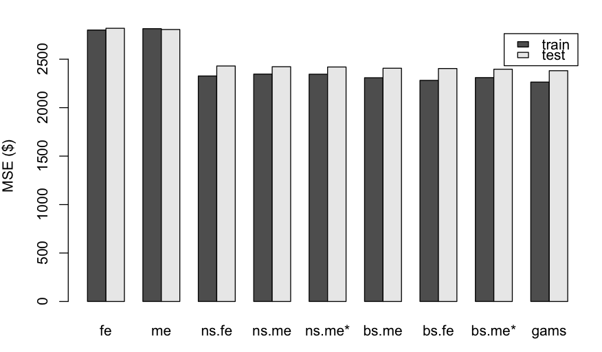
The following figure shows the train and test errors obtained when fitting each model to a training set consisting of a stratified 80% sample of the original dataset. We compare the log-linear model to three basis-function models: one using cubic b-splines [(bs) function in R ], another using natural cubic splines [(ns) function in R] and a third using a Generalized Additive model [(gam) function from the (mgcv) package]. For the first three models, we compare the Fixed Effect [(fe) suffix] and the Mixed Effect [(me) suffix] versions.
 |
|---|
| Train and Test MSE for each of the models under consideration [(fe): log-linear fixed effects model, (me): log-linear mixed effects model, (bs.fe/me): b-splines fixed/mixed effects, (ns.fe/me): natural cubic splines fixed/mixed effects, (gams) generative additive model from R’s (mgcv) package. The ME models with the $*$ superscript impose a diagonal structure on the random effects covariance $\Sigma$. ] |
There’re a few things that stand out from these results. First, we see that the basis function models we introduced have helped improve both errors by over 10% with respect to the original log-linear models [labeled (fe) and (me) in the figure]. Second, we also see that the difference between the mixed effect and fixed effect alternatives is very small, and both alternatives match the performance of the (gams) model [which is also a Fixed Effects one according to our convention]. This came as a surprise to me, given the popular knowledge that ME models should show superior performance under small sample sizes for one or more of the groups. On the contrary, these results show that for this dataset we wouldn’t profit from mixed effects models at all, since we would get similar predictive performance by fitting a simple polynomial spline or a gam model to each car model’s data independently. Of course if our main goal was interpretation more so than predictive power, mixed effect models provide some information that the others won’t a priori be able to capture.
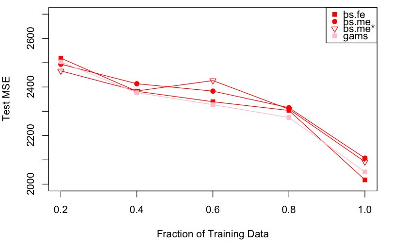
But the question intrigued me enough that I wrote another experiment to evaluate the performance of the Fixed Effects and Mixed Effects alternatives as a function of the size of the training data. My hypothesis was that there was a regime where the additional structure imposed by the Mixed Effects model would result into superior predictive performance. The results of this experiment, where I evaluated test MSE over multiple runs on a subset of training data of varying size, are shown in the figure below:
 |
|---|
| Test MSE for four of the models under consideration [(bs.fe/me): b-splines fixed/mixed effects, (gams) generative additive model from R’s (mgcv) package. It’s hard to argue that Mixed Effects models have any advantage over the alternatives.] |
It seems then that even with a fraction of 20% only of the training data [about 420 samples only], the mixed effects variants don’t show any significant advantage over the fixed effects alternatives. It is not clear to me why this is the case, especially for the diagonal covariance [(bs.me*)] model, with smaller degrees of freedom and more structure than the independent, fixed effects model one. But the data shows what it shows, and I don’t have any more time to investigate this rebellious behavior…
So what are the depreciation rates after all?
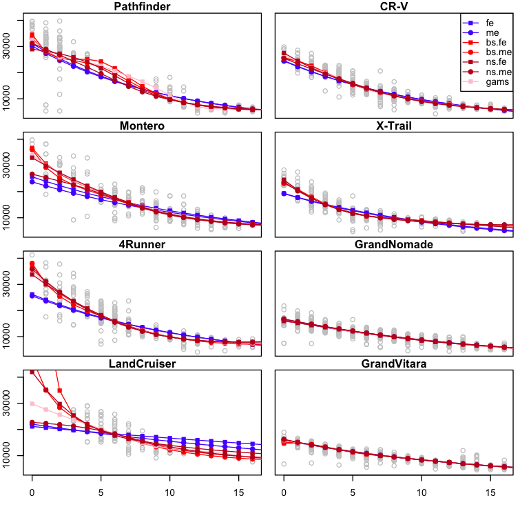
It’s easy for a data scientist to go down the rabbit hole of model building and checking and loose sight of the original question that motivated the modeling work. But I haven’t forgotten: my main goal here was to estimate the depreciation rates for each car model, and see if there was some insight that could inform our purchase decision. So let’s have a look at the fit for each model under the assumption that all the model variables are fixed except for age [here the y-axis correponds to price in USD, x-axis to age in years]:
 |
|---|
| Fitted values [price in USD, y-axis] for each of the considered models as a function of Age [x-axis], when leaving all other covariates fixed. [(fe): log-linear fixed effects model, (me): log-linear mixed effects model, (bs.fe/me): b-splines fixed/mixed effects, (ns.fe/me): natural cubic splines fixed/mixed effects, (gam s) generative additive model from R’s (mgcv) package.] |
The fits look pretty similar among all the non-linear models we have been experimenting with, except for strong variations in the boundary areas [small and large age values]. This is not surprising since each model imposes different boundary conditions and the amount of samples near the extremes is smaller [remember the histograms from the previous post?]. But what we are interested in are the depreciation rates, so let’s plot those as a function of age:
 |
|---|
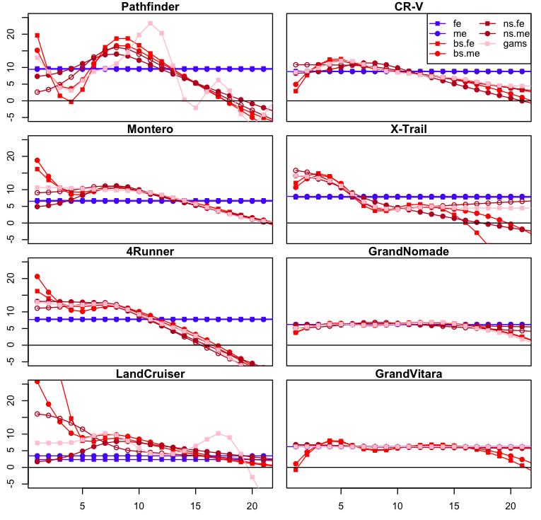
| Depreciation [in %, y-axis] as a function of age [x-axis], for each of the models under consideration. [(fe): log-linear fixed effects model, (me): log-linear mixed effects model, (bs.fe/me): b-splines fixed/mixed effects, (ns.fe/me): natural cubic splines fixed/mixed effects, (gam s) generative additive model from R’s (mgcv) package.] |
The differences between each statistical model become now a lot clearer. We see for instance that the log-linear model tends to underestimate the depreciation that occurs early in the lifetime of a car, while overestimating the devaluation that takes place later. What’s interesting from this chart, more so than the discrepancies between each non-linear model, is in fact the agreement in the shape that the depreciation rate takes over time. [It would be great if we could quantify the uncertainty around these curves to statistically justify this last statement, but the current implementation of mixed models in R pretty much renders it impossible. More on this later!] There seem to be in fact two classes of depreciation rate profiles: one, illustrated by the car models on the left side of the figure, corresponds to a large depreciation in the beginning that tapers down until about 5 years, when it increases again to peak a little before the 10 year mark. The other, corresponding to the right side, starts low to peak at around year 4 to then peter out slowly. These are very qualitative observations, but it would be interesting to gather more evidence on whether these two depreciation patterns occur for other car models or other products in general.
Finally, I found it surprising that both Suzuki models display the steadiest depreciation rate. I could especulate endlessly about the reasons behind this, but all I can say for the moment is that this behavior doesn’t seem to be due a model artifact. Nonetheless, I wouldn’t discount the possibility that the the profiles for the other models come with significantly larger error bars due to their smaller sample size.
So why don’t you calculate the damn error bars?
The short answer is: because I’m lazy. The longer answer is that I don’t know of any R package that provides principled error bars for mixed effect models in reasonable time [that is, other than by bootstrapping means.]
According to the (lme4) package documentation [2], the main reason why the package doesn’t provide prediction error bands is that it is hard to incorporate the errors from the model’s covariance estimates.
So short of letting my laptop spend days running parametric bootstrap simulationsof the mixed model predictions, I decided that this was a great opportunity to try out Stan, the probabilistic programming language that is becoming increasingly popular for Bayesian analyses. More about it soon!
References
[1] The elements of statistical learning, Trevor Hastie, Robert Tibshirani, Jerome Friedman
[2] Package ‘lme4’ documentation
Source code
The charts in this blog post have been generated with these scripts: nonlinear.R, meVsFe.R.