Dorfman's group testing with uncertainty

Arnau Tibau-Puig, arnau dot tibau at gmail dot com, May 10th, 2020

The source code generate this page and its figures can be found in Github: github.com/atibaup/group-testing

Note: This is part II of my blog post on "Group testing for prevalence estimation and disease monitoring".

Introduction

In my previous post, we discussed Dorfman's (2-stage) Group Testing strategy, whose setup can be quickly summarized by the following figure:

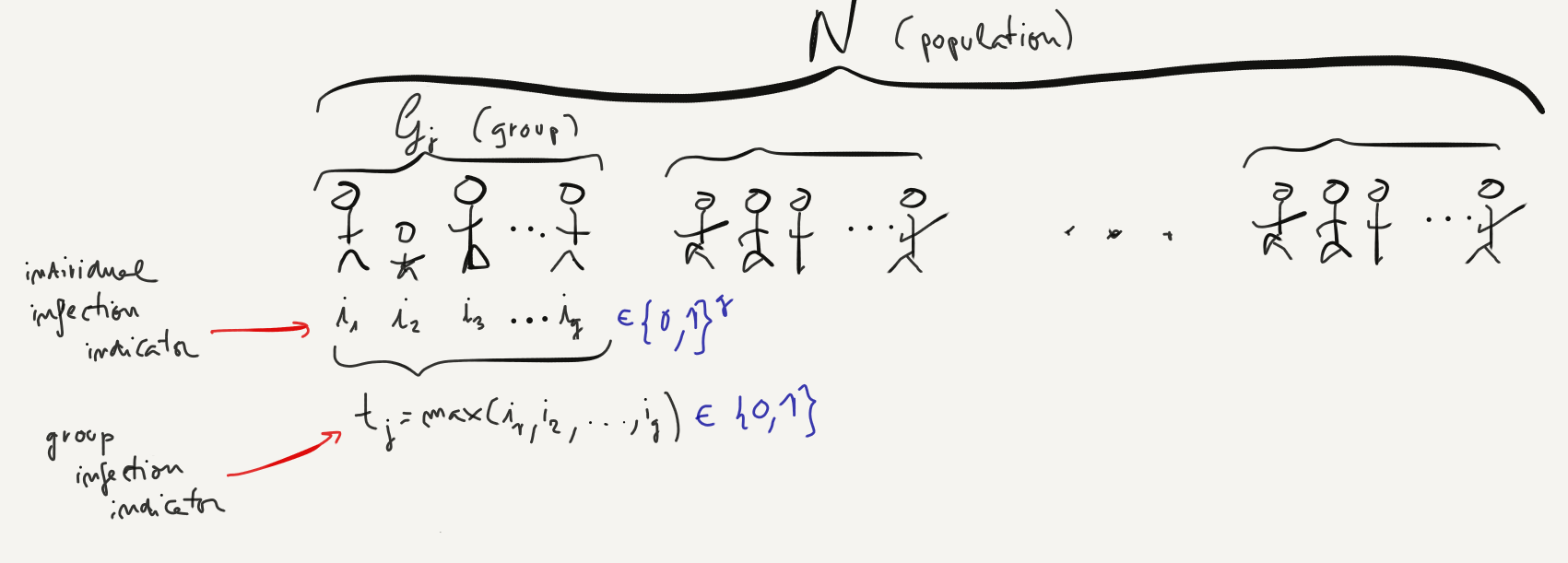
Under that simplified setup, where we assumed that our test was errorless (that is, it generated no false negatives or false positives), we showed that one could obtain substantial efficiencies by applying the following group testing (also known as pooled testing) strategy:

1. Divide the population into groups of $g$ individuals
2. For each group, draw a specimen from each individual and pool them together.
3. Run the test on the pooled sample. If the test turns positive, test each of the $g$ individuals in the pool, running a total of $g+1$ tests for that pool. Otherwise, if the test turns negative, label the $g$ individuals as non-infected.

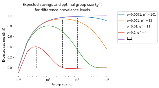
In particular, Dorfman showed that we could detect individuals infected with a low-prevalence disease with only a fraction of the tests needed to test individually the whole population. For example, for a disease with a prevalence of 1%, we could identify the infected individuals by only running 1/5th of the tests necessary to test the whole population. In other words, if we have a limited number of tests, we could screen 5 times as many people:

However, during the derivation of the above charts, we hid a couple of important details under the rug:

1. We assumed that the testing procedure was errorless, and
2. That the test results within and across groups were statistically independent.

In this post we relax the first assumption and consider the situation were the test procedure is noisy, under a pretty generic statistical model of test errors. Of course this topic has already received some attention in the abundant group testing literature, see for example [1] for a recent review on the results obtained so far under the assumption of negligible or no dilution effect. For the study of errors induced by dilution of the sample, [2] considered a model of error under the dilution of limited practical appeal. The approach described here is closer to that of [3], derived in the context of analyzing dilution in pooled samples for HIV screening.

Characterizing noisy tests

In the original Dorfman setup, it is implicitly assumed that there exist a methodology to, given a sample from an individual or a group of individuals, determine whether the sample contains the biomarker of interest, say, a syphilis antigen. This is what we call an errorless or noiseless test: a test that perfectly identifies the presence or absence of a given biomarker, without error.

In practice this is an unrealistic assumption: almost all tests that depend on measuring physical quantities are subject to (at least) measurement error, and hence they are not perfect. Luckily, modelling decision-making under uncertainty has been the bread and butter of statistics for almost 100 years.

To characterize a test with error, we will need to define two additional quantities:

• a test statistic, which we will usually denote by a random variable $s$,
• a decision threshold, which we will denote by a deterministic value $\eta$.

The test statistic is typically a function of the quantity we measure. For example, in the Real Time-Polymerase Chain Reaction (RT-PCR) assays used to detect the presence of viral RNA in a sample, the test statistic is a function of the number of thermocycles needed for the fluorescence of a sample to exceed a given threshold. This statistic is a (non-linear) function of the underlying quantitiy of interest, which is the concentration of viral RNA.

Given an observation for the test statistic, $s$, we can then define the outcome of the test as a Bernouilli random variable $t$ defined as follows:

$t = \left\{\begin{array}{cc} 1 & s\geq \eta \\ 0 & \mbox{otherwise}\end{array}\right.$,

With this notation at hand, we are ready to characterize the statistical error that ensues from the fact that $s$ is a non-deterministic quantity. To do so, we typically define two quantities:

• The Specificity, which we will denote by $\pi_0$ and define as $\pi_0 = P\left(t = 0 | i = 0 \right)$, the probability of discarding an infection if the individual is healthy,

• The Sensitivity, which we will denote by $\pi_1$ and define as $\pi_1 = P\left(t = 1 | i = 1 \right)$, the probability of detecting an infection if the individual is infected.

Remember that in our setup $i$ denotes whether an individual is really infected or not, that is, the "ground truth".

Note that our original errorless tests are a special case of this model, where both the sensitivity and the specificity are equal to $1$. That is the same as saying that there are no false negatives or false positives. On the other hand, when there is uncertainty, it is often impossible to achieve both perfect sensitivity and specificity. As we become more sensitive in detecting positives, increasing the sensitivity, we will have to accept a few false positives, that is, a decrease in specificity.

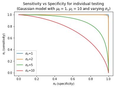
In order to better understand how these quantities evolve as a function of the amount of uncertainty, we plot below the behavior of these quantities as a function of $\eta$ and a specific instance of our model where $s | i \sim \mathcal{N}\left(\mu_{i}, \sigma_q\right)$. As we can see, swapping over $\eta$ generates a curve of $\pi_0$ and $\pi_1$, also known as Receiver Operating Characteristic (ROC). The Area Under the Curve (AUC) is a measure of how much error a test displays - the higher the variance the lower the Area Under the Curve.

Group testing with uncertainty

Before we formalize the problem set up, it can be healthy to ask ourselves what do we expect to happen when we start using a noisy testing procedure with pooled samples... Would we expect the expected number of tests to increase or decrease? Do we expect the amount of false positives/negatives to be larger or smaller than the individual testing strategy?

At first sight, it's hard to imagine how errors could help in any way. But it's also easy to show that a noisy testing procedure could actually reduce the expected number of tests, though at the expense of increasing the false negative rate. To see this, consider the extreme case of a test with zero specificity, which always rejects all groups. We will only perform $\frac{N}{g}$ tests, but we will have a terrible false negative rate (we won't identify any infection!). This very simple line of reasoning seems to suggest that errors can increase or decrease both the number of tests we end up performing as well as the performance of our estimates.

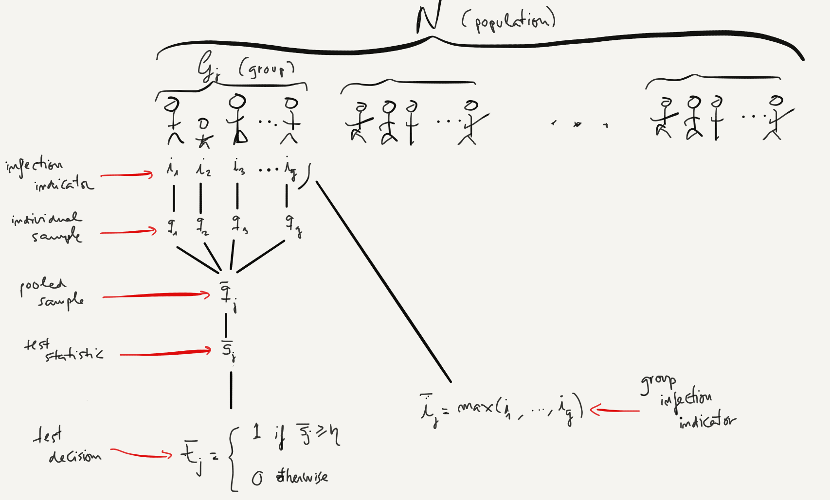
Let's setup the problem now. We will need to expand the individual testing notation from the previous section and define:

• $\bar{i}_k$: a Bernouilli random variable denoting whether anyone in the group is infected or not, which we can analytically define as $\bar{i}_k = \max_{j \in \mathcal{G}_k} i_j$.
• $\bar{q}_k$: a real-valued random variable corresponding to the measurement of a bio-marker for the pooled sample corresponding to group $k$. In general, $\bar{q}_k$ will be a function of $q_j, j \in \mathcal{G}_k$.
• $\bar{s}_k$: the group test statistic, which we will assume to take the form $\bar{s}_k = f(\bar{q}_k, \epsilon)$ where $f$ is deterministic and $\epsilon$ is iid noise.
• $\bar{t}_k$: the group test outcome, a Bernouilli random variable defined as follows:

$\bar{t}_k= \left\{\begin{array}{cc} 1 & \bar{s}_k\geq \bar{\eta} \\ 0 & \mbox{otherwise}\end{array}\right.$,

where $\bar{\eta}$ is now the group decision threshold. Similar to the last section, we can now characterize the statistical performance of one group test by defining its:

• Group-Specificity, which we will denote by $\bar{\pi}_0$ and define as $\bar{\pi}_0 = P\left(\bar{t} = 0 | \bar{i}_k = 0 \right)$, that is, the probability of discarding a group if the whole group is healthy, and

• Group-Sensitivity, which we will denote by $\bar{\pi}_1$ and define as $\bar{\pi}_1 = P\left(\bar{t} = 0 | \bar{i}_k = 1\right)$, that is, the probability of detecting a group positive if at least one individual in the group is infected.

The following diagram can serve as a quick reference of the group testing setup and notation (compare to the diagram of Dorfman's original setup in the Introduction):

Impact of dilution on group-specificity and group-sensitivity

The first question we want to study is how the specificity and sensitivity of the pooled test are impacted by the dilution of a "positive" (infected) sample in a pool of $g-1$ "healthy" samples. At first sight, it seems that diluting an infected sample shouldn't help its group-sensitivity... Consider the extreme case where the group is so big that the concentration of the infected biomarker becomes negligible and thus it is impossible to detect anything.

In order to gain more understanding without resorting to computational tools, we will make a few additional simplifying assumptions:

1. We will assume that, conditional on the infection indicator, the biomarker measurements follow a Normal distribution $q_j | i_j \sim \mathcal{N}\left(\mu_{i_j}, \sigma_q\right)$ parameterized by $\mu_0, \mu_1$ and $\sigma_q$.
2. We will also assume that the pooled biomarker measurement is equal to the average of biomarker measurements in the pool, that is $\bar{q}_k = \frac{1}{g}\sum_{j \in \mathcal{G}_k} q_j$
3. We will also assume that both the group and individual testing statistics, are defined by the following relation $s = f\left(q\right)$ where $f$ is a monotonic function of its argument.

Note that the last two assumptions seem reasonable: On one hand, if we are measuring concentrations of a given biomarker in a sample, when mixing the samples we would expect the resulting concentration to be the average of each member in the pool. On the other, a well-behaved test statistic should evolve montonically with the concentration of interest.

Under these additional assumptions we can define the group-specificity as:

$\bar{\pi}_0 = P\left(\bar{t} = 0 | \bar{i}_k = 0 \right) = P\left(\bar{s}_k < \bar{\eta} | \bar{i}_k = 0 \right) = P\left(f(\bar{q}_k) < \bar{\eta} | \bar{i}_k = 0 \right) = P\left(\bar{q}_k < f^{-1}\left(\bar{\eta}\right) | \bar{i}_k = 0 \right)$

Since the individuals in the group have been chosen uniformly at random, it is fair to expect the quantities $q_j, j \in \mathcal{G}_k$ to be independent of each other, which allows us to conclude that:

$\bar{q}_k | \bar{i}_k = 0 \sim \mathcal{N}\left(\mu_{0}, \frac{1}{\sqrt{g}}\sigma_q\right)$,

where we have used the property that the sum of two normally distributed random variables is normally distributed with mean and variance equal to the sum of means and variances of each summand, respectively. As a consequence, if we set the group-threshold at $\bar{\eta}$, we have:

$\bar{\pi}_0 = P\left(\bar{q}_k | \bar{i}_k = 0 \right) = P\left( q_j < f^{-1}\left(\bar{\eta}\right) | i_j = 0 \right) = \phi\left(\sqrt{g}\left(\frac{f^{-1}\left(\bar{\eta}\right) - \mu_0}{\sigma_q}\right)\right)$

where $\phi\left(x\right)$ is the cumulative distribution function of the Standard Normal. Note that in order to obtain the same group-specificity as the specificity of an individual test, we would need to set the group threshold such that:

$\sqrt{g}\left(\frac{f^{-1}\left(\bar{\eta}\right) - \mu_0}{\sigma_q}\right) = \frac{f^{-1}\left(\eta\right) - \mu_0}{\sigma_q}$

which means that in such case the group-threshold should be set at:

$\bar{\eta} = f\left(\frac{f^{-1}\left(\eta\right) - \mu_0}{\sqrt{g}} + \mu_0 \right)$

On the other hand, we define the group-sensitivity as:

$\bar{\pi}_1 = P\left(\bar{t} = 1 | \bar{i}_k = 1 \right) = P\left(\bar{s}_k \geq \bar{\eta} | \bar{i}_k = 1 \right) = P\left(\bar{q}_k \geq f^{-1}\left(\bar{\eta}\right) | \bar{i}_k = 1 \right)$

This expression is trickier to evaluate because there are several combinations of $\left\{i_j, j \in \mathcal{G}_k\right\}$ that correspond to $\bar{i}_k = 1$. The good news is that, given the individual-to-individual independence of $q_j$, and letting $0 \leq m_k = \sum_{j\in \mathcal{G}_k} i_j \leq g$ denote the number of infected individuals in group $\mathcal{G}_k$, we can easily characterize $\bar{q}_k$ as:

$\bar{q}_k | m_k \sim \mathcal{N}\left(\mu\left(g, n\right), \frac{\sigma_q}{\sqrt{g}}\right)$

where, for convenience, we define:

$\mu\left(g, n\right) = \frac{1}{g}\left(\left(g - n\right)\mu_{0} + n \mu_{1}\right)$,

and we have again leveraged standard properties of independent Normal random variables. On the other hand, since $\left\{i_j\right\}_{j\in \mathcal{G}_k}$ are iid, we also have that $m_k$ is a Binomial random variable:

$P\left(m_k = m\right) = {g \choose m} p^m\left(1 - p\right)^{g-m}$,

and hence:

$\bar{\pi}_1 = \sum_{m=1}^g P\left(\bar{q}_k \geq f^{-1}\left(\bar{\eta}\right) | \bar{i}_k = 1, m_k=m\right)P\left(m_k=m | m_k \geq 1\right) = \sum_{m=1}^g\left(1 -\phi\left(\sqrt{g}\left(\frac{f^{-1}\left(\bar{\eta}\right) - \mu\left(g, m\right)}{\sigma_q}\right)\right)\right)P\left(m_k=m | m_k \geq 1\right)$

where:

$P\left(m_k=m | m_k \geq 1\right) = \frac{P\left(m_k \geq 1 | m_k=m\right)P\left(m_k=m\right)}{P\left(m_k \geq 1\right)} = \left\{\begin{array}{cc} \frac{1}{1 - \left(1 - p\right)^{g}}{g \choose m} p^m\left(1 - p\right)^{g-m} & m>0 \\ 0 & m=0\end{array}\right.$

Note that for small enough $p$,

$P\left(m_k=1 | m_k \geq 1\right) \approx 1$

and $\bar{\pi}_1$ can be approximated as:

$\bar{\pi}_1 \approx 1 - \phi\left(\sqrt{g}\left(\frac{f^{-1}\left(\bar{\eta}\right) - \mu\left(g, 1\right)}{\sigma_q}\right)\right)$

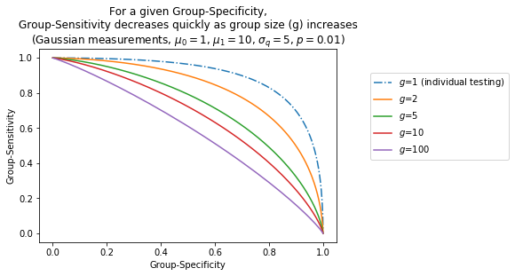
The following figure characterizes the degradation of $\bar{\pi}_1$ as a function of $p$ and $g$, under the simplified model we have used throughout this section:

Impact of noise on the number of tests performed

We have reasoned earlier that noisy tests can both reduce or increase the number of tests we need to perform under Dorfman's two-stage procedure. Let's attempt now to characterize that quantity, as well as the savings relative to an individual testing strategy, when the tests have known group-sentitivity and group-specificity, denoted by $\bar{\pi}_1$ and $\bar{\pi}_0$.

Following the same reasoning we used in the first post, under an inter-group independence assumption, the expected number of tests performed is now given by:

$E\left(T'\right) = E\left(\sum_{n=1}^{N/g} I_{\bar{t}_n=1}\left(g + 1\right) + I_{\bar{t}_n=0} \right) = \frac{n}{g}\left(\left(1- P_0'\right)\left(g + 1\right) + P_0'\right)$

where we use $T'$ to indicate the number of tests necessary in the presence of test errors, to differentiate it from the number of tests $T$ in the errorless setting, and where $P_0'$ denotes the probability of the group-test turning negative:

$P_0' = E\left(I_{\bar{t}_n=0}\right) = P\left(\bar{t}_n=0\right)$,

which under the presence of noise, is now a function of $\bar{\pi}_1$ and $\bar{\pi}_0$:

$P_0' = P\left(\bar{t}_n=0 | \bar{i}_n = 0\right)P\left(\bar{i}_n = 0\right) + P\left(\bar{t}_n=0 | \bar{i}_n = 1\right)P\left(\bar{i}_n = 1\right) = \bar{\pi}_0 P_0 + \left(1 - \bar{\pi}_1\right)\left(1 - P_0\right)$

where we have let $P_0=P\left(\bar{i}_n = 0\right) = \left(1 - p\right)^g$ (provided again we have intra-group independence between the individuals).

We can also define the savings relative to the individual testing strategy and calculate its expectation:

$E\left(\gamma'\right) = 1 - \frac{g + 1}{g}\left(1 - P_0'\right) - \frac{1}{g}P_0'$

Let's explore the dependency of $E\left(\gamma'\right)$ on $p$, $g$ and $\bar{\pi}_1$ and $\bar{\pi}_0$:

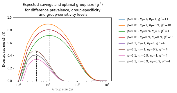
It is clear from the figure that the presence of noise can both increase or decrease the expected savings from applying a group-testing procedure. In general, decreasing the group-sensitivity ($\bar{\pi}_1$) will result in higher savings, as we will see next at the expense of a larger false negative rate. On the other hand, a decrease in the specificity will result in smaller savings, as well as a larger amount of false positives. Interestingly, when $\bar{\pi}_0=\bar{\pi}_1$ we have that

$P_0' = \bar{\pi}_0 P_0 + \left(1 - \bar{\pi}_1\right)\left(1 - P_0\right) = P_0$

and hence, in this special case, the amount of savings and optimal group size is the same as in the noiseless case, $E\left(\gamma'\right)=E\left(\gamma\right)$.

Global specificity and sensitivity

So far we have been able to characterize the group-sensitivity and group-specificity of the first stage in Dorfman's group test procedure. We have also used that characterization to understand the expected savings in number of tests ($E(\gamma')$) relative to an individual testing strategy, as well as the optimal group size in the presence of test noise.

We still haven't said anything yet about the global sensitivity and specificity at the end of the 2-stage Dorfman group-testing procedure. To do so, we will need to introduce once again some additional notation. We will identify by $t'_j$ the test outcome for individual $j$ at the end of the second stage, as illustrated by the diagram below:

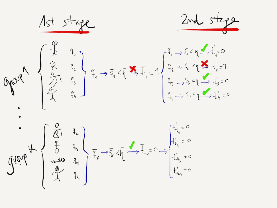
As illustrated in the diagram above, according to Dorfman's procedure, an individual will test positive ($t'_j=1$) if both the first stage group-test for her group is positive ($\bar{t}_k=1$) and the second stage test is positive ($t_j=1$). Otherwise the individual will test negative:

$t'_j = \left\{ \begin{array}{cc} 1 & \mbox{ if } \bar{t}_k=1, t_j=1 \\ 0 & \mbox{ if } \bar{t}_k=0 \mbox{ or } \bar{t}_k=1, t_j=0\end{array}\right.$

This allows us to characterize the global specificity of the 2-stage procedure ($\pi_0'$) as:

$\pi_0' = P\left(t'_j=0 | i_j=0 \right) = P\left(t'_j=0 | i_j=0, \bar{t}_k=0 \right)P\left(\bar{t}_k=0 | i_j=0 \right) + P\left(t'_j=0 | i_j=0, \bar{t}_k=1 \right)P\left(\bar{t}_k=1 | i_j=0 \right)$

Looking at each term on the right hand side individually, we see that two of them can be explicitly calculated:

• $P\left(t'_j=0 | i_j=0, \bar{t}_k=0 \right) = 1$, because according to the procedure, the individual is automatically assumed to be a negative if the group-test turns negative,
• $P\left(t'_j=0 | i_j=0, \bar{t}_k=1 \right) = P\left(t'_j=0 | i_j=0\right) = \pi_0$ because the outcome of the second test is independent of $\bar{t}_k=1$, conditional on $i_j=0$, where $\pi_0$ is the specificit of an individual test.

Thus we can calculate $\pi_0'$ as:

$\pi_0' = P\left(\bar{t}_k=0 | i_j=0 \right) + \pi_0 P\left(\bar{t}_k=1 | i_j=0 \right)$

which allows us to conclude that $\pi_0 \leq \pi_0'\leq 1$, which means that the global specificity of Dorfam's 2-stage procedure can be no worse than that of individual testing.

Similarly, we can also characterize the global specificity of the 2-stage procedure ($\pi_1'$) as:

$\pi_1' = P\left(t'_j=1 | i_j=1 \right) = P\left(t'_j=1 | i_j=1, \bar{t}_k=0 \right)P\left(\bar{t}_k=0 | i_j=1 \right) + P\left(t'_j=1 | i_j=1, \bar{t}_k=1 \right)P\left(\bar{t}_k=1 | i_j=1 \right)$

where we can identify:

• $P\left(t'_j=1 | i_j=1, \bar{t}_k=0 \right)=0$,
• $P\left(t'_j=1 | i_j=1, \bar{t}_k=1 \right)=P\left(t'_j=1 | i_j=1 \right)=\pi_1$, the sensitivity of an individual test.

By construction of the second stage and conditional independence properties, leading to:

$\pi_1' = \pi_1 P\left(\bar{t}_k=1 | i_j=1 \right)$

which implies that $0 \leq \pi_1' \leq \pi_1$, meaning that the global sensitivity can be only as good as that of the individual test ($\pi_1$). Put together, these two observations suggests that in practice, applying Dorfman's group testing could improve the specificity but deteriorate the sensitivity, which makes sense since in order to test positive, a sample will need to clear two hurdles (the group and the individual test) instead of just one (the individual test).

Global specificity and sensitivity in a simple Gaussian model

To get any further in characterizing $\pi_0'$ and $\pi_1'$, we would need specific models for the quantities $P\left(\bar{t}_k | i_j \right)$, appearing in $\pi_0'$ and $\pi_1'$. So let's explore what happens in the following special case:

1. The biomarker measurements follow a Normal distribution $q_j | i_j \sim \mathcal{N}\left(\mu_{i_j}, \sigma_q\right)$ parameterized by $\mu_0, \mu_1$ and $\sigma_q$.
2. The pooled biomarker measurement is equal to the average of biomarker measurements in the pool, that is $\bar{q}_k = \frac{1}{g}\sum_{j \in \mathcal{G}_k} q_j$
3. The group and individual test statistics are defined by the following relation $s = f\left(q\right)$ where $f$ is a monotonic function of its argument.

First, we observe that we can characterize $P\left(\bar{t}_k | i_j \right)$ as:

$P\left(\bar{t}_k=x | i_j=y \right) = \sum_{n=0}^{g}P\left(\bar{t}_k=x | i_j=y, m_j=n \right)P\left(m_j=n| i_j=y\right)$

where we have defined an auxiliary random variable $m_j = \sum_{i\in \mathcal{G}_k \backslash j} i_i$ corresponding to the number of infected individuals in the same group as individual $j$, excluding $j$ itself. By virtue of the fact that the indivual infection indicators $i_j$ in a group are assumed to be statistically independent, we can see that:

$P\left(m_j=n| i_j\right) = P\left(m_j=n\right) = {g-1 \choose n} p^n\left(1 - p\right)^{g-1-n}$

where $p$ is the probability of any single individual being infected.

With this in hand, we now only need to worry about the $P\left(\bar{t}_k=x | i_j=y, m=n \right)$ piece. Using the model assumptions (1)-(3) above, we can see that:

$P\left(\bar{t} = 0 | i_j=x, m_j=n \right) = P\left(\bar{s}_k < \bar{\eta} | i_j=x, m_j=n \right) = P\left(f(\bar{q}_k) < \bar{\eta} | i_j=x, m_j=n\right) = P\left(\bar{q}_k < f^{-1}\left(\bar{\eta}\right) | i_j=x, m_j=n\right)$

and that we have

$\bar{q}_k | i_j, m_j=n \sim \mathcal{N}\left(\mu\left(i_j, n\right), \frac{\sigma_q}{\sqrt{g}}\right)$

where

$\mu\left(i_j=0, n\right) = \frac{1}{g}\left(\left(g - n\right)\mu_{0} + n \mu_{1}\right)$

corresponds to the average biomarker measurement when individual $j$ is not infected ($i_j=0$), and $n$ of its group "neighbors" are infected, and:

$\mu\left(i_j=1, n\right) = \frac{1}{g}\left(\left(g - 1 - n\right)\mu_{0} + \left(n + 1\right)\mu_{1}\right)$

corresponds to the average biomarker measurement when individual $j$ is infected ($i_j=1$), and $n$ of its group "neighbors" are also infected.

So in fact we can just compute $P\left(\bar{t} = 0 | i_j=x, m_j=n \right)$ from the Cumulative Distribution Function (cdf) of a Normal variable with mean given by the two expressions above. A similar result can be obtained for $P\left(\bar{t} = 1 | i_j=x, m_j=n \right)$ simply by reverting the inequality from $\bar{q}_k < f^{-1}\left(\bar{\eta}\right)$ to $\bar{q}_k \geq f^{-1}\left(\bar{\eta}\right)$.

We are now ready to explore what the global sensitivity and specificity look like as a function of the group size and the test statistic thresholds $\eta$ and $\bar{\eta}$, for a model where $\mu_0 = -20$, $\mu_1 = 20$, $\sigma_q = 30$, $g=10$ and $p = 0.01$.

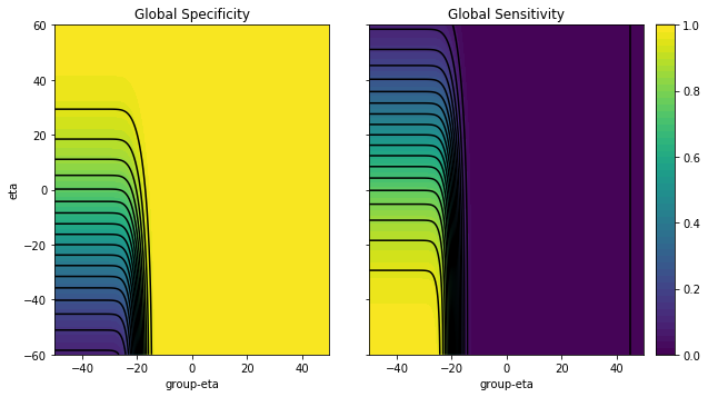
The figures above show that, as one would expect, the global specificity increases as we increase the first and second stage tresholds, while the global sensitivity decreases.

In addition, it also shows that one needs to be careful about choosing both the 1st and 2nd stage thresholds ($\eta$ and $\bar{\eta}$, respectively). Choosing either one sloppily can lead to disastrous results:

• If for instance, we set too large a $\bar{\eta}$ in the example above, we would be getting perfect specificity, but zero sensitivity, no matter what value we set the second stage threshold $\eta$ to.
• On the other hand, if we set too high a $\eta$, no matter what value we choose for $\bar{\eta}$, we would also be rejecting all tests, achieving high specificity but zero sensitivity.

For now we don't yet have a simple criterion to select the thresholds $\bar{\eta}, \eta$. One approach would be to define a priori a specificity level we are comfortable with, say at $\pi_0'=0.95$, which defines a set $S\left(\pi_0'\right):=\left\{\bar{\eta}, \eta\right\}$ of first and second stage thresholds that correspond to that sensitivity, and find that set computationally:

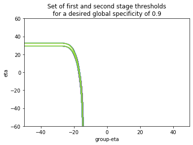
To finally choose the operating point that maximizes the sensitivity at that global specificity level:

$\max_{\bar{\eta}, \eta \in S\left(\pi_0'\right)} \pi_1'$

However this approach would ignore the effect on the expected number of tests, which we characterized earlier in terms of the group-specificity ($\bar{\pi}_0$) and group-sensitivity ($\bar{\pi}_1$). As we saw in the section "Impact of noise on the number of tests performed", decreasing specificity will typically increase the number of expected tests we will need to run, because of the increasing false group positives. So perhaps a more compelling approach would be to:

1. Set a desired global specificity level
2. Pick $\bar{\eta}, \eta$ such that we find a good balance between the global-sensitivity ($\pi_1'$), and the expected savings in number of tests performed ($E(\gamma')$).

Conclusions

In this post we have characterized Dorfman's two stage group testing in a noisy setting where we assume both the tests at the first (group) stage and the second (individual) stage are susceptible to make errors.

We have seen that:

1. We can characterize the expected number of tests in this setup as a function of the group-specificity and the group-sensitivity. As expected, the number of tests will increase with lower specificity, and decrease with lower sensitivity.
2. We have also characterized the effect of dilution on these quantities in a simple model that allows us to model the impact in the group-ROC as the group size increases
3. We have characterized the global performance of the two-stage procedure, in terms of the global-specificity and the global-sensitivity, which depend on the first and second stage thresholds. We have characterized this performance in a simple Gaussian model and suggested a strategy to pick the operating thresholds.

In a subsequent blog post we will investigate the second assumption underlying Dorfman's group testing: "The independence of the individuals within a group, as well as independence of the test's outcome across groups".

Acknowledgements

I would like to thank Aleix Ruiz Villa for reading a draft of this post and spotting a couple of errors, as well as Pere Puig for sharing a few references and fruitful email exchanges on the topic of group testing.

References

[1] Comparison of Group Testing Algorithms for Case Identification in the Presence of Test Error, Hae-Young Kim et al.

[2] Group testing with a dilution effect , F. K. Hwang

[3] Pooled Testing for HIV Screening: Capturing the Dilution Effect, L. M. Wein, S. A. Zenios